Simulating Stock Prices: A Monte Carlo Approach
The main objective of this project to predict the plausible range of NVDA stock price based on historical data. We will use 10 years of historical data.
Imports and Initial Setup
import numpy as np
import pandas as pd
import yfinance as yf
import matplotlib.pyplot as plt
from scipy.stats import norm
%matplotlib inline
Data Extraction
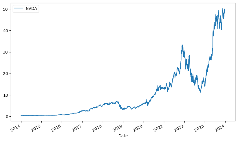
The first step involves extracting historical stock price data for NVIDIA Corp (NVDA) from Yahoo Finance. The ticker variable specifies the stock symbol, and the yf.download function fetches the adjusted closing prices over a specified period (January 1, 2014, to January 1, 2024). This data is stored in a pandas DataFrame and plotted to visualize the stock price trend over the selected period. In finance, historical stock prices are fundamental for understanding past performance and making future predictions.
ticker = 'NVDA'

stock_data = pd.DataFrame()
stock_data[ticker] = yf.download(ticker, start='2014-1-1', end='2024-1-1')['Adj Close']

stock_data.plot(figsize=(10,6));
Calculate Historical Log Returns
Log returns are calculated using the natural logarithm of the percentage change in stock prices. This transformation is common in finance because log returns have desirable statistical properties, such as normality, which simplify further analysis. The log returns are then plotted to visualize their behavior and distribution. Understanding the distribution of returns is essential for assessing the risk and volatility of a stock, which are critical factors in financial decision-making.
log_returns = np.log(1 + stock_data.pct_change())
log_returns.plot(figsize=(10,6))
log_returns.plot.density();
Statistical Measures
Next the mean, variance, and standard deviation of the log returns were calculated. These statistical measures provide insights into the average return, variability, and risk associated with the stock. In finance, these metrics help investors understand the expected performance and potential fluctuations in stock prices, aiding in portfolio management and risk assessment. I will need these values to calculate drift later in our project.
mean = log_returns.mean()
variance = log_returns.var()
STD = log_returns.std()
Simulate Future Daily Returns and Prices
Monte Carlo simulations are used to predict future stock prices. The code sets the number of trading days (‘t_intervals’) and the number of simulations (‘simulations’). It then generates random daily log returns based on the historical standard deviation and converts them to simple returns. The shape of the simulated returns array is checked to ensure it matches the expected dimensions. This process models the randomness and uncertainty inherent in financial markets, providing a range of possible future outcomes.
t_intervals = 250
simulations = 10000

daily_logreturns_simulated = STD.values * norm.ppf(np.random.rand(t_intervals, simulations))
daily_simplereturns_simulated = np.exp(daily_logreturns_simulated)
daily_simplereturns_simulated.shape
Calculate Future Prices
Next we initialized the future price list with the latest known stock price and uses a loop to calculate future prices based on the simulated returns. This simulation generates multiple possible price paths for the stock over the specified period. Plotting these paths helps visualize the potential future trajectories of the stock price, giving investors a sense of the range and likelihood of different outcomes.
last_price = stock_data.iloc[-1]
price_list = np.zeros_like(daily_simplereturns_simulated)
price_list[0] = last_price

for t in range(1, t_intervals):
    price_list[t] = price_list[t-1] * daily_simplereturns_simulated[t]

plt.plot(price_list);
Quantifications
I then calculated the worst, average, and best-case scenarios for the stock price at the end of the simulation period. It also computes confidence intervals (1 and 2 standard deviations) to quantify the uncertainty in the predictions. These results provide a range of potential future prices and the likelihood of different outcomes, helping investors make informed decisions based on their risk tolerance and investment goals.
WorstSim = round(price_list[-1].min(), 2)
AvgSim = round(price_list[-1].mean(), 2)
BestSim = round(price_list[-1].max(), 2)

print('Best and Worst Cases')
print(f'Worst Simulation $/share: {WorstSim}')
print(f'Average Simulation $/share: {AvgSim}')
print(f'Best Simulation $/share: {BestSim}')

Mean_Day250Prices = price_list[-1].mean()
SD_Day250Prices = price_list[-1].std()
UpperInterval_1SD = Mean_Day250Prices + 1 * SD_Day250Prices
LowerInterval_1SD = Mean_Day250Prices - 1 * SD_Day250Prices
UpperInterval_2SD = Mean_Day250Prices + 2 * SD_Day250Prices
LowerInterval_2SD = Mean_Day250Prices - 2 * SD_Day250Prices

print('\n' + 'Confidence Intervals')
print(f'1 Sigma (1 S.D.): 68% confident that price after 250 days will fall between ${round(LowerInterval_1SD,2)} and ${round(UpperInterval_1SD,2)}')
print(f'2 Sigma (2 S.D.): 95% confident that price after 250 days will fall between ${round(LowerInterval_2SD, 2)} and ${round(UpperInterval_2SD, 2)}')
Results of the Simulations
The results of the Monte Carlo simulation for NVIDIA's stock price reveal a wide range of potential outcomes. The worst-case scenario predicts the stock could drop to $13.69 per share, while the best-case scenario suggests it could soar to $432.41 per share, with an average simulation resulting in a price of $80.44 per share. Additionally, the confidence intervals provide further insight: there is a 68% confidence that the stock price after 250 days will fall between $41.72 and $119.16 (1 Sigma), and a 95% confidence that it will range between $3.0 and $157.88 (2 Sigma). These intervals help quantify the uncertainty and variability in the stock's future performance.
Results: Best and Worst Cases
Worst Simulation $/share: 13.69
Average Simulation $/share: 80.44
Best Simulation $/share: 432.41

Confidence Intervals
1 Sigma (1 S.D.): 68% confident that price after 250 days will fall between $41.72 and $119.16
2 Sigma (2 S.D.): 95% confident that price after 250 days will fall between $3.0 and $157.88


